The Fourier transform, named after Joseph Fourier, is a mathematical transform with many applications in physics and engineering. Very commonly it transforms a mathematical function of time, f(t), into a new function, sometimes denoted by or F, whose argument is frequency with units of cycles/s (hertz) or radians per second. The new function is then known as the Fourier transform and/or the frequency spectrum of the function f. The Fourier transform is also a reversible operation. Thus, given the function one can determine the original function, f. (See Fourier inversion theorem.) f and are also respectively known as time domain and frequency domain representations of the same "event". Most often perhaps, f is a real-valued function, and is complex valued, where a complex number describes both the amplitude and phase of a corresponding frequency component. In general, f is also complex, such as the analytic representation of a real-valued function. The term "Fourier transform" refers to both the transform operation and to the complex-valued function it produces.
In the case of a periodic function (for example, a continuous but not necessarily sinusoidal musical sound), the Fourier transform can be simplified to the calculation of a discrete set of complex amplitudes, called Fourier series coefficients. Also, when a time-domain function is sampled to facilitate storage or computer-processing, it is still possible to recreate a version of the original Fourier transform according to the Poisson summation formula, also known as discrete-time Fourier transform. These topics are addressed in separate articles. For an overview of those and other related operations, refer to Fourier analysis or List of Fourier-related transforms.
When the independent variable x represents time (with SI unit of seconds), the transform variable ξ represents frequency (in hertz). Under suitable conditions, f is determined by ƒ̂ via the inverse transform:
for every real number x.
The statement that f can be reconstructed from ƒ̂ is known as the Fourier inversion theorem, and was first introduced in Fourier'sAnalytical Theory of Heat (Fourier 1822, p. 525), (Fourier & Freeman 1878, p. 408), although what would be considered a proof by modern standards was not given until much later (Titchmarsh 1948, p. 1). The functions f and ƒ̂ often are referred to as a Fourier integral pair or Fourier transform pair (Rahman 2011, p. 10).
The Fourier transform relates the function's time domain, shown in red, to the function's frequency domain, shown in blue. The component frequencies, spread across the frequency spectrum, are represented as peaks in the frequency domain.
The motivation for the Fourier transform comes from the study of Fourier series. In the study of Fourier series, complicated but periodic functions are written as the sum of simple waves mathematically represented by sines and cosines. The Fourier transform is an extension of the Fourier series that results when the period of the represented function is lengthened and allowed to approach infinity.(Taneja 2008, p. 192)
Due to the properties of sine and cosine, it is possible to recover the amplitude of each wave in a Fourier series using an integral. In many cases it is desirable to use Euler's formula, which states that e2πiθ= cos(2πθ) + isin(2πθ), to write Fourier series in terms of the basic waves e2πiθ. This has the advantage of simplifying many of the formulas involved, and provides a formulation for Fourier series that more closely resembles the definition followed in this article. Re-writing sines and cosines as complex exponentials makes it necessary for the Fourier coefficients to be complex valued. The usual interpretation of this complex number is that it gives both the amplitude (or size) of the wave present in the function and the phase (or the initial angle) of the wave. These complex exponentials sometimes contain negative "frequencies". If θ is measured in seconds, then the waves e2πiθ and e−2πiθ both complete one cycle per second, but they represent different frequencies in the Fourier transform. Hence, frequency no longer measures the number of cycles per unit time, but is still closely related.
There is a close connection between the definition of Fourier series and the Fourier transform for functions f which are zero outside of an interval. For such a function, we can calculate its Fourier series on any interval that includes the points where f is not identically zero. The Fourier transform is also defined for such a function. As we increase the length of the interval on which we calculate the Fourier series, then the Fourier series coefficients begin to look like the Fourier transform and the sum of the Fourier series of f begins to look like the inverse Fourier transform. To explain this more precisely, suppose that T is large enough so that the interval [−T/2,T/2] contains the interval on which f is not identically zero. Then the n-th series coefficient cn is given by:
Comparing this to the definition of the Fourier transform, it follows that cn = ƒ̂(n/T) since f(x) is zero outside [−T/2,T/2]. Thus the Fourier coefficients are just the values of the Fourier transform sampled on a grid of width 1/T. As T increases the Fourier coefficients more closely represent the Fourier transform of the function.
Under appropriate conditions, the sum of the Fourier series of f will equal the function f. In other words, f can be written:
where the last sum is simply the first sum rewritten using the definitions ξn = n/T, and Δξ = (n + 1)/T − n/T = 1/T.
This second sum is a Riemann sum, and so by letting T → ∞ it will converge to the integral for the inverse Fourier transform given in the definition section. Under suitable conditions this argument may be made precise (Stein & Shakarchi 2003).
In the study of Fourier series the numbers cn could be thought of as the "amount" of the wave present in the Fourier series of f. Similarly, as seen above, the Fourier transform can be thought of as a function that measures how much of each individual frequency is present in our function f, and we can recombine these waves by using an integral (or "continuous sum") to reproduce the original function.
The following images provide a visual illustration of how the Fourier transform measures whether a frequency is present in a particular function. The function depicted f(t) = cos(6πt) e-πt2 oscillates at 3 hertz (if t measures seconds) and tends quickly to 0. (The second factor in this equation is an envelope function that shapes the continuous sinusoid into a short pulse. Its general form is a Gaussian function). This function was specially chosen to have a real Fourier transform which can easily be plotted. The first image contains its graph. In order to calculate ƒ̂(3) we must integrate e−2πi(3t)f(t). The second image shows the plot of the real and imaginary parts of this function. The real part of the integrand is almost always positive, because when f(t) is negative, the real part of e−2πi(3t) is negative as well. Because they oscillate at the same rate, when f(t) is positive, so is the real part of e−2πi(3t). The result is that when you integrate the real part of the integrand you get a relatively large number (in this case 0.5). On the other hand, when you try to measure a frequency that is not present, as in the case when we look at ƒ̂(5), the integrand oscillates enough so that the integral is very small. The general situation may be a bit more complicated than this, but this in spirit is how the Fourier transform measures how much of an individual frequency is present in a function f(t).
Original function showing oscillation 3 hertz.
Real and imaginary parts of integrand for Fourier transform at 3 hertz
Real and imaginary parts of integrand for Fourier transform at 5 hertz
The Fourier transform translates between convolution and multiplication of functions. If f(x) and g(x) are integrable functions with Fourier transforms and respectively, then the Fourier transform of the convolution is given by the product of the Fourier transforms and (under other conventions for the definition of the Fourier transform a constant factor may appear).
Conversely, if f(x) can be decomposed as the product of two square integrable functions p(x) and q(x), then the Fourier transform of f(x) is given by the convolution of the respective Fourier transforms and .
Denoting the Fourier transform by a capital letter corresponding to the letter of function being transformed (such as f(x) and F(ξ)) is especially common in the sciences and engineering. In electronics, the omega (ω) is often used instead of ξ due to its interpretation as angular frequency, sometimes it is written as F(jω), where j is the imaginary unit, to indicate its relationship with the Laplace transform, and sometimes it is written informally as F(2πf) in order to use ordinary frequency.
The interpretation of the complex function ƒ̂(ξ) may be aided by expressing it in polar coordinate form
in terms of the two real functions A(ξ) and φ(ξ) where:
which is a recombination of all the frequency components of f(x). Each component is a complex sinusoid of the form e2πixξ whose amplitude is A(ξ) and whose initial phase angle (at x = 0) is φ(ξ).
The Fourier transform may be thought of as a mapping on function spaces. This mapping is here denoted and is used to denote the Fourier transform of the function f. This mapping is linear, which means that can also be seen as a linear transformation on the function space and implies that the standard notation in linear algebra of applying a linear transformation to a vector (here the function f) can be used to write instead of . Since the result of applying the Fourier transform is again a function, we can be interested in the value of this function evaluated at the value ξ for its variable, and this is denoted either as or as . Notice that in the former case, it is implicitly understood that is applied first to f and then the resulting function is evaluated at ξ, not the other way around.
In mathematics and various applied sciences it is often necessary to distinguish between a function f and the value of f when its variable equals x, denoted f(x). This means that a notation like formally can be interpreted as the Fourier transform of the values of f at x. Despite this flaw, the previous notation appears frequently, often when a particular function or a function of a particular variable is to be transformed.
For example, is sometimes used to express that the Fourier transform of a rectangular function is a sinc function,
or is used to express the shift property of the Fourier transform.
Notice, that the last example is only correct under the assumption that the transformed function is a function of x, not of x0.
The Fourier transform can also be written in terms of angular frequency: ω = 2πξ whose units are radians per second.
The substitution ξ = ω/(2π) into the formulas above produces this convention:
Under this convention, the inverse transform becomes:
Unlike the convention followed in this article, when the Fourier transform is defined this way, it is no longer a unitary transformation on L2(Rn). There is also less symmetry between the formulas for the Fourier transform and its inverse.
Another convention is to split the factor of (2π)n evenly between the Fourier transform and its inverse, which leads to definitions:
Under this convention, the Fourier transform is again a unitary transformation on L2(Rn). It also restores the symmetry between the Fourier transform and its inverse.
Variations of all three conventions can be created by conjugating the complex-exponential kernel of both the forward and the reverse transform. The signs must be opposites. Other than that, the choice is (again) a matter of convention.
Summary of popular forms of the Fourier transform
ordinary frequency ξ (hertz)
unitary
angular frequency ω (rad/s)
non-unitary
unitary
As discussed above, the characteristic function of a random variable is the same as the Fourier–Stieltjes transform of its distribution measure, but in this context it is typical to take a different convention for the constants. Typically characteristic function is defined .
As in the case of the "non-unitary angular frequency" convention above, there is no factor of 2π appearing in either of the integral, or in the exponential. Unlike any of the conventions appearing above, this convention takes the opposite sign in the exponential.
The following tables record some closed form Fourier transforms. For functions f(x), g(x) and h(x) denote their Fourier transforms by ƒ̂, , and respectively. Only the three most common conventions are included. It may be useful to notice that entry 105 gives a relationship between the Fourier transform of a function and the original function, which can be seen as relating the Fourier transform and its inverse.
This shows that, for the unitary Fourier transforms, the Gaussian function exp(−αx2) is its own Fourier transform for some choice of α. For this to be integrable we must have Re(α)>0.
Here, n is a natural number and is the n-th distribution derivative of the Dirac delta function. This rule follows from rules 107 and 301. Combining this rule with 101, we can transform all polynomials.
309
Here sgn(ξ) is the sign function. Note that 1/x is not a distribution. It is necessary to use the Cauchy principal value when testing against Schwartz functions. This rule is useful in studying the Hilbert transform.
This formula is valid for 0 > α > −1. For α > 0 some singular terms arise at the origin that can be found by differentiating 318. If Re α > −1, then is a locally integrable function, and so a tempered distribution. The function is a holomorphic function from the right half-plane to the space of tempered distributions. It admits a unique meromorphic extension to a tempered distribution, also denoted for α ≠ −2, −4, ... (See homogeneous distribution.)
312
The dual of rule 309. This time the Fourier transforms need to be considered as Cauchy principal value.
313
The function u(x) is the Heaviside unit step function; this follows from rules 101, 301, and 312.
314
This function is known as the Dirac comb function. This result can be derived from 302 and 102, together with the fact that
as distributions.
315
The function J0(x) is the zeroth order Bessel function of first kind.
To 400: The variables ξx, ξy, ωx, ωy, νx and νy are real numbers.
The integrals are taken over the entire plane.
To 401: Both functions are Gaussians, which may not have unit volume.
To 402: The function is defined by circ(r)=1 0≤r≤1, and is 0 otherwise. This is the Airy distribution, and is expressed using J1 (the order 1 Bessel function of the first kind). (Stein & Weiss 1971, Thm. IV.3.3)
Formulas for general n-dimensional functions[edit]
Function
Fourier transform unitary, ordinary frequency
Fourier transform unitary, angular frequency
Fourier transform non-unitary, angular frequency
500
501
502
503
Remarks
To 501:
The function χ[0,1] is the indicator function of the interval [0, 1]. The function Γ(x) is the gamma function. The function Jn/2 + δ is a Bessel function of the first kind, with order n/2 + δ. Taking n = 2 and δ = 0 produces 402. (Stein & Weiss 1971, Thm. 4.15)
To 502:
See Riesz potential. The formula also holds for all α ≠ −n, −n − 1, ... by analytic continuation, but then the function and its Fourier transforms need to be understood as suitably regularized tempered distributions. See homogeneous distribution.
To 503:
This is the formula for a multivariate normal distribution normalized to 1 with a mean of 0. Bold variables are vectors or matrices. Following the notation of the aforementioned page, and
Bracewell, R. N. (2000), The Fourier Transform and Its Applications (3rd ed.), Boston: McGraw-Hill, ISBN0-07-116043-4.
Campbell, George; Foster, Ronald (1948), Fourier Integrals for Practical Applications, New York: D. Van Nostrand Company, Inc..
Condon, E. U. (1937), "Immersion of the Fourier transform in a continuous group of functional transformations", Proc. Nat. Acad. Sci. USA, 23: 158–164.
Duoandikoetxea, Javier (2001), Fourier Analysis, American Mathematical Society, ISBN0-8218-2172-5.
Fourier, J. B. Joseph; Freeman, Alexander, translator (1878), The Analytical Theory of Heat, The University Press {{citation}}: |first2= has generic name (help)CS1 maint: multiple names: authors list (link)
Grafakos, Loukas (2004), Classical and Modern Fourier Analysis, Prentice-Hall, ISBN0-13-035399-X.
Hewitt, Edwin; Ross, Kenneth A. (1970), Abstract harmonic analysis. Vol. II: Structure and analysis for compact groups. Analysis on locally compact Abelian groups, Die Grundlehren der mathematischen Wissenschaften, Band 152, Berlin, New York: Springer-Verlag, MR0262773.
Titchmarsh, E (1948), Introduction to the theory of Fourier integrals (2nd ed.), Oxford University: Clarendon Press (published 1986), ISBN978-0-8284-0324-5.
Wilson, R. G. (1995), Fourier Series and Optical Transform Techniques in Contemporary Optics, New York: Wiley, ISBN0-471-30357-7.


.gif)


 Original function showing oscillation 3 hertz.
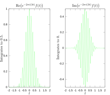 Real and imaginary parts of integrand for Fourier transform at 3 hertz
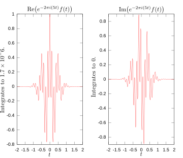 Real and imaginary parts of integrand for Fourier transform at 5 hertz
 Fourier transform with 3 and 5 hertz labeled.


![{\displaystyle \displaystyle \chi _{[0,1]}(|x|)(1-|x|^{2})^{\delta }}](https://wikimedia.org/api/rest_v1/media/math/render/svg/6c42190ce04a2aacb193c4460aab695ee32ec977)


